Advanced features of Pychastic¶

Multiple starting positions¶

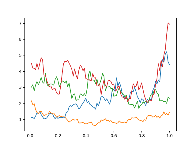
Sometimes we are interested in equilibrium properties of studied system. It is beneficial to pick different initial conditions for each sample path in such way that starting condition is distributed according to equilibrium configuration. Such behaviour is accomplished setting x0 value in SDEProblem to a list of initial conditions and setting n_trajectories to None (setting n_trajectories to a different value raises an `ValueError)

import jax
import matplotlib.pyplot as plt
from pychastic.sde_solver import SDESolver
from pychastic.sde_problem import SDEProblem

solver = SDESolver(scheme="milstein", dt=1e-2)

a = 1
b = 1
problem = SDEProblem(
    a=lambda x: a * x,
    b=lambda x: b * x,
    x0=1.0,
    tmax=1.0,
    exact_solution=lambda x0, t, w: x0 * np.exp((a - 0.5 * b * b) * t + b * w),
)

problem.x0 = jax.numpy.array([[1.],[2.],[3.],[4.]])

result = solver.solve_many(problem, n_trajectories=None)

for (t,x) in zip(result['time_values'],result['solution_values']):
    plt.plot(t,x)

plt.show()

Memory management - sample discarding¶

In many cases (for example stiff equations) even though small step is required we are not really interested in values at all steps. We can use this to our advantage by discarding evaluation points which are not needed. You can accompish this behaviour using chunk_size option of solve and solve_many methods.

Memory management - randomization discarding¶

It is much more efficient to compute all random values in advance and not generate noise at each step. Sadly this comes at memory cost. By default all randomization is done before integrating trajectories, we can split this process into smaller runs by using chunks_per_randomization option of solve and solve_many methods.

Step post-processing aka domain hacks¶

Whenever we are anaysing SDE or ODE on a manifold whose universal cover is not \(\mathbb{R}^n\) we need to handle switching between charts. Similarily, if we know that some constraint is satisfied exactly in our system (conservation of energy or momentum for example) we overcome error accumulation in conserved variables by projecting onto desired subspace after each step. Both of those needs can be acomplished using step_post_processing option of solve and solve_many methods. It takses a function which maps location in phase space onto adjusted new location in phase space after each step.

# Following code simulates rigid body rotations (dynamics on SO(3)) for more details
# check our paper https://arxiv.org/abs/2209.04332
import pychastic
import jax.numpy as jnp
import jax
import matplotlib.pyplot as plt
import numpy as np

mobility = 2.0*jnp.eye(3)
mobility_d = jnp.linalg.cholesky(mobility) # Compare with equation: Evensen2008.6

def spin_matrix(q):
    # Antisymmetric matrix dual to q
    return jnp.array([[0, -q[2], q[1]], [q[2], 0, -q[0]], [-q[1], q[0], 0]])


def rotation_matrix(q):
    # Compare with equation: Evensen2008.11
    phi = jnp.sqrt(jnp.sum(q ** 2))
    rot = (
        (jnp.sin(phi) / phi) * spin_matrix(q)
        + jnp.cos(phi) * jnp.eye(3)
        + ((1.0 - jnp.cos(phi)) / phi ** 2) * q.reshape(1, 3) * q.reshape(3, 1)
    )
    return jax.lax.cond(phi > 0.01, lambda: rot, lambda: 1.0 * jnp.eye(3))


def transformation_matrix(q):
    # Compare with equation: Evensen2008.12
    phi = jnp.sqrt(jnp.sum(q ** 2))
    trans = (
        0.5
        * (1.0 / phi ** 2 - (jnp.sin(phi) / (2.0 * phi * (1.0 - jnp.cos(phi)))))
        * q.reshape(1, 3)
        * q.reshape(3, 1)
        + spin_matrix(q)
        + (phi * jnp.sin(phi) / (1.0 - jnp.cos(phi))) * jnp.eye(3)
    )
    return jax.lax.cond(phi > 0.01, lambda: trans, lambda: 1.0 * jnp.eye(3))


def metric_force(q):
    # Compare with equation: Evensen2008.10
    phi = jnp.sqrt(jnp.sum(q ** 2))
    scale = jax.lax.cond(
        phi < 0.01,
        lambda t: -t / 6.0,
        lambda t: jnp.sin(t) / (1.0 - jnp.cos(t)) - 2.0 / t,
        phi,
    )
    return jax.lax.cond(
        phi > 0.0, lambda: (q / phi) * scale, lambda: jnp.array([0.0, 0.0, 0.0])
    )


def t_mobility(q):
    # Mobility matrix transformed to coordinates.
    # Compare with equation: Evensen2008.2
    return transformation_matrix(q) @ mobility @ (transformation_matrix(q).T)


def drift(q):
    # Drift term.
    # Compare with equation: Evensen2008.5
    # jax.jacobian has differentiation index last (like mu_ij d_k)
    # so divergence is contraction of first and last axis.
    return t_mobility(q) @ metric_force(q) + jnp.einsum(
        "iji->j", jax.jacobian(t_mobility)(q)
    )


def noise(q):
    # Noise term.
    # Compare with equation: Evensen2008.5
    return jnp.sqrt(2) * transformation_matrix(q) @ (rotation_matrix(q).T) @ mobility_d


def canonicalize_coordinates(q):
    phi = jnp.sqrt(jnp.sum(q ** 2))
    max_phi = jnp.pi
    canonical_phi = jnp.fmod(phi + max_phi, 2.0 * max_phi) - max_phi
    return jax.lax.cond(
        phi > max_phi,
        lambda canonical_phi, phi, q: (canonical_phi / phi) * q,
        lambda canonical_phi, phi, q: q,
        canonical_phi,
        phi,
        q,
    )


problem = pychastic.sde_problem.SDEProblem(
    drift, noise, tmax=20.0, x0=jnp.array([1.0, 0.0, 0.0])
)

solver = pychastic.sde_solver.SDESolver(dt=0.01)

trajectories = solver.solve_many(
    problem,
    step_post_processing=canonicalize_coordinates,
    n_trajectories=1000,
    chunk_size=100,
    chunks_per_randomization=1,
)

final_angles = np.array(
    jnp.sqrt(jnp.sum(trajectories["solution_values"][:, -1, :] ** 2, axis=1))
)

Pychastic for derivatives pricing

Examples