Pychastic for molecular simulations¶

Introduction - why bother?¶

Molecular dynamics finds applications in physics, material science, structural biology and others. Main problem with making MD simulations is that ODEs governing the systems are very stiff due to timescale disparity. One of shortest timescales is viscosity mediated relaxation of solvents. There are generally two ways of dealing with it – explicit solvent and bigger supercomputer or implicit solvent and often lack of hydrodynamic interactions. In either case estimating diffusive properties of molecules is near impossible.

Small DNA loop undergoing Brownian dynamics

About 0.5 millisecond of Brownian motion of twisted DNA loop of length 1000 angstroms.¶

(Note millisecond not microsecond like in typical MD simulations).

Here SDEs come to rescue – correct formulation of overdamped dynamics reduces order of ODEs to first order with stochastic noise removing shortest timescale from the simulations. Additionally in Stokesian regime hydrodynamic interactions can be introduced via mobility matrices.

Mathematical setting¶

In the following sections we’ll be solving SDE of one or two variables. They’re most commonly written in differential form. Ito calculus is a little different than typical real valued calculus in that functions we’re working with (such as Wiener processes realisations) are almost surely nowhere differentiable, this is reflected in the notation by refusal to write expressions like \(dW/dt\).

Typical problem setting would look like:

\[dX = a dt + b dW\]

Here \(dX\) represents change in value we’re tracking, \(a dt\) is systematic drift of our process and \(b dW\) is noise term.

Sphere’s Brownian motion near a wall¶

Simplest nontrivial example of Brownian dynamics is suspension of noninteracitng spheres in diffusion-sedimentation balance. It is exactly the setting under investigation in the famous 1905 paper by A. Einstein.

If we measure distance in multiples of particles radius and time in multiples of \(R^2 / 2 k_b T \mu_\infty\) and energies in multiples of \(k_b T\) the equation becomes:

\[dh = \frac{\partial_h \mu(h)}{2} dt + \frac{\mu(h)}{\mu_\infty}\partial_h U(h) dt + \sqrt{2\frac{\mu(h)}{\mu_\infty}} dW\]

where \(\mu(h)\) is the height dependent mobility function and \(U(h)\) is height dependent potential energy.

In the simplest approximation we can take:

\[ \begin{align}\begin{aligned}U(h) = g h\\\mu(h) / \mu_\infty = 1 - 1/h\end{aligned}\end{align} \]

This way mobility goes to zero at contact with the wall and approaches bulk value far from the wall.

High performance code thanks to `jax.jit`¶

Python code can be slow and when simulating SDEs we’ll be evaluating coefficient functions thousands of times. The solution to the issue is just in time compilation or jit. It allows users to still write python code, but compiles it to machine code when necessary to make it comparably fast to C code.

Second problem we encounter in numerical solution of SDEs is the need to compute gradients. Fortunately we don’t need to manually type in derivatives and higher derivatives of all functions we’re using. jax.grad is a package that can figure out derivatives of functions as long as they are built from familiar blocks such as sin cos or pow functions.

Amazingly we can have both at the same time – jax is a package designed precisely with this in mind. Originally designed to accelerate gradient computations in machine learning it will suit us just fine.

If it all sounds too good to be true you’re partially right. All of this acceleration and gradients comes at expense of giving up some functionality of numpy. In jax all arrays are immutable which allows for keeping track of all function applications.

Essentially, to have gradients, you need to program functionally.

In most cases we’ve encountered it’s not a big problem since the equations usually come from mathematical or physical background where notation reflects functional, rather than imperative, mindset.

You can learn more how to code better in jax in their tutorial.

Simulating scalar SDEs¶

(If you want to enjoy plots as well you’ll need matplotlib package)

import pychastic
import jax.numpy as np #to make jit acceleration possible
g = 2.0 # units are [k_b T / sphere size]
problem = pychastic.sde_problem.SDEProblem(
    lambda x: (1.0 / x**2) - (1.0-1.0/x)*g,
    lambda x: np.sqrt(2.0*(1.0-1.0/x)),
    1.5,
    50.0
    )
solver = pychastic.sde_solver.SDESolver()
trajectory = solver.solve(problem)
trajectory
{'time_values': array([0.000e+00, 1.000e-02, ..., 5.001e+01]),
'solution_values': array([1.5, 1.49303699, ..., nan]),
'wiener_values': array([ 0., 0.01052365, ...])} #some values are random
import matplotlib.pyplot as plt
plt.plot(trajectory['time_values'],trajectory['solution_values'])
plt.show()

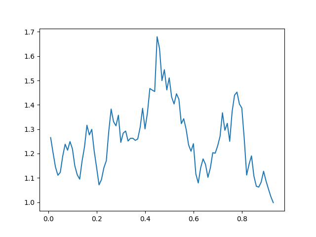
The SDEProblem constructor takes two callables (functions) as arguments. First one describes the drift term, second one describes the noise term. In python you can define functions either by using def keyword or on-the-fly using lambda keyword like we did here.

We’re using a slightly different flavor of numpy that being jax.numpy this variant is compatible with just-in-time compilation which greatly increases code speed (often to the same order of magnitude as C code).

Finally as you can see solution values starts with sensible numbers but from some point it’s filled with nan values. This is because of taking square root of negative value – we’ve intersected the wall! This is an issue with time step being too large you can fix this by setting smaller timestep and better integration method either in SDESolver constructor or in solver.dt later (but before calling solve!)

Generating many trajectories¶

It’s not uncommon that we’re interested in a whole ensemble of trajectories. Because of jit optimization it’s much faster to generate trajectories together rather than one at a time (considerable time is spent pre-compiling coefficient functions, but this ideally happens only once).

import pychastic
import jax.numpy as np
g = 2.0
problem = pychastic.sde_problem.SDEProblem(
    lambda x: (1.0 / x**2) - (1.0-1.0/x)*g,
    lambda x: np.sqrt(2.0*(1.0-1.0/x)),
    1.5,
    0.5
    )
solver = pychastic.sde_solver.SDESolver(dt = 0.001)
trajectories = solver.solve_many(problem,500)
import matplotlib.pyplot as plt
plt.hist(trajectories['solution_values'][:,-1].flatten())
plt.show()

#### TODO ##### Improve example, add histogram and shaded plot with confidence bands and such.

More degrees of freedom¶

All of the above is neat but it’s been well understood for a couple of decades now. Most likely you’d want to simulate many particles or at least one particle that can rotate and move in all three dimensions.

Unless you’re really lucky and the problem separates into separate equations for each of the directions you’ll need to integrate all degrees of freedom simultaneously. It can be accomplished using vector SDEs.

Simulating vector SDEs¶

This section relies on package pygrpy for hydrodynamic interactions. You can get it via pip by

python3 -m pip install pygrpy

We’ll be relying on pygrpy.jax_grpy_tensors.muTT functionality to get mobility matrices in Rotne-Prager-Yakamava approximation.

Mobility matrices connect forces and velocities on particles via relation:

\[v_{ai} = \mu_{abij} F_{bj}\]

Where indices \(a,b\) go through spheres id and indices \(i,j\) through spatial dimensions.

Given the \(\mu\) tensor we can express dynamics of all spheres as

\[dX_{ai} = \mu_{abij} \partial_{bj} U(X) dt + \sqrt{2 k_b T \mu_{abij}} dW_{ai} + k_bT \partial_{bj} \mu_{abij} dt\]

Where \(U\) denotes potential energy dependent on locations of all beads. It turns out that Rotne-Prager-Yakamawa is particularly convenient for us as the last term including divergence vanishes.

For now we’ll simulate two beads connected by a spring of rest length 4.0. We’ll work in natural units where energy is measured in multiples of \(k_bT\) and distances in multiples of sphere’s radii. This convention can be summarized with the following table.

Quantity	Scale (measured as multiple of)
Distance	\(L\)
Time	\(\eta L^3 / k_b T\)
Energy	\(k_b T\)
Force	\(k_b T / L\)

We can go ahead and code this equation in python.

import pychastic                   # solving sde
import pygrpy.jax_grpy_tensors     # hydrodynamic interactions
import jax.numpy as jnp            # jax array operations
import jax                         # taking gradients
import matplotlib.pyplot as plt    # plotting
radii = jnp.array([1.0,0.2]) # sizes of spheres we're using
def u_ene(x): # potential energy shape
     locations = jnp.reshape(x,(2,3))
     distance = jnp.sqrt(jnp.sum((locations[0] - locations[1])**2))
     return (distance-4.0)**2

def drift(x):
     locations = jnp.reshape(x,(2,3))
     mu = pygrpy.jax_grpy_tensors.muTT(locations,radii)
     force = -jax.grad(u_ene)(x)
     return jnp.matmul(mu,force)

def noise(x):
     locations = jnp.reshape(x,(2,3))
     mu = pygrpy.jax_grpy_tensors.muTT(locations,radii)
     return jnp.sqrt(2)*jnp.linalg.cholesky(mu)

problem = pychastic.sde_problem.SDEProblem(
      drift,
      noise,
      x0 = jnp.reshape(jnp.array([[0.,0.,0.],[0.,0.,4.]]),(6,)),
      tmax = 500.0)
solver = pychastic.sde_solver.SDESolver()
trajectory = solver.solve(problem) # takes about 10 seconds
plt.plot(trajectory['time_values'],trajectory['solution_values'][:,0])
plt.plot(trajectory['time_values'],trajectory['solution_values'][:,3])
plt.show()

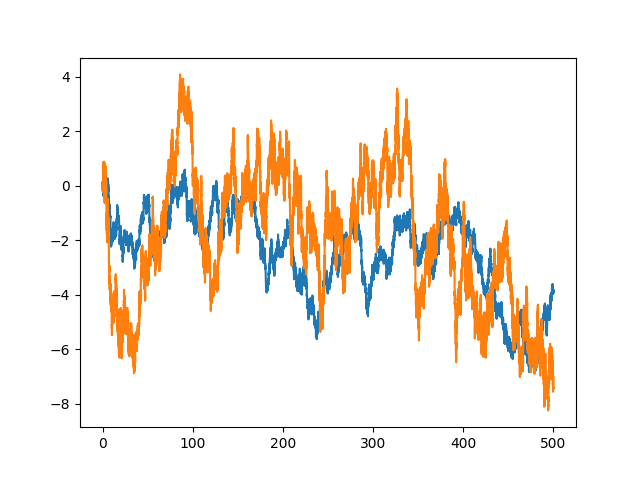
_images/tutorial_brownian_twospheres.png

As you can see first sphere’s (blue) trajectory is less noisy than seconds sphere’s trajectory, as expected. Smaller shere gets bounced around much more than large sphere. Additionally, even though their motion appears independent on short timescales they stay together because they are connected by a spring.

You’re good to go! There are many options that control the integration precision and speed. You can choose different algorithms for integration as well.

One large and one small bead moving according to Brownian motion

3D animation of the two spheres connected with harmonic spring example.¶