Examples
This page highlights some possible use cases of Pychastic package.
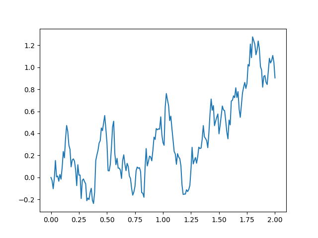
Simple Brownian motion
Brownain motion of a particle in one dimension is where SDE’s started. In this example there is no drift and noise is constant
import pychastic
import jax.numpy as jnp
problem = pychastic.sde_problem.SDEProblem(lambda x: jnp.array(1.0),lambda x: jnp.array(1.0),0.0,2.0)
solver = pychastic.sde_solver.SDESolver()
trajectory = solver.solve(problem)
trajectory
{'time_values': array([0.,0.01,...]), 'solution_values' : array([0.,0.0082,...]),'wiener_values' : array([0.,0.0082,...])} #some values random
import matplotlib.pyplot as plt
plt.plot(trajectory['time_values'],trajectory['solution_values'])
plt.show()
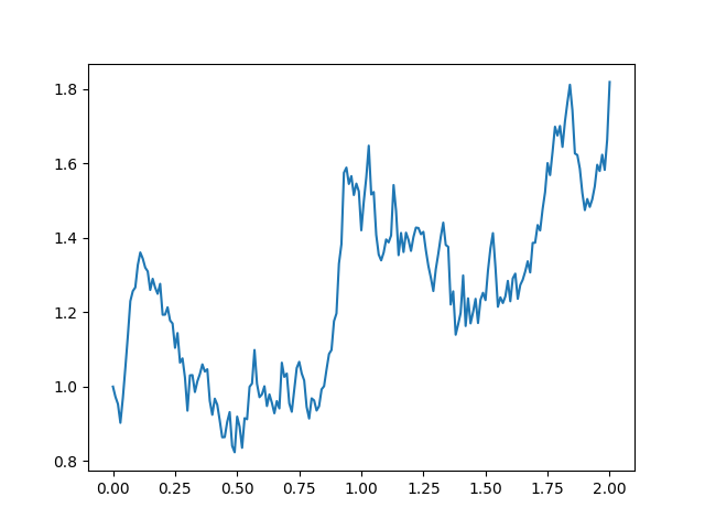
Geometric Brownian motion
In this classic example both drift and noise are proportional to current value. Such process is used as model for stock market behaviour.
import pychastic
problem = pychastic.sde_problem.SDEProblem(lambda x: 0.2*x,lambda x: 0.5*x,1.0,2.0)
solver = pychastic.sde_solver.SDESolver()
trajectory = solver.solve(problem)
import matplotlib.pyplot as plt
plt.plot(trajectory['time_values'],trajectory['solution_values'])
plt.show()