Pychastic for derivatives pricing
Introduction - why bother?
The Black-Sholes formula has a closed form expression, so we’re done for pricing european options. Well not really. If you’re here you probably have heared of stochastic volitality models, or want to price more exotic instruments, these do not have closed form expressions for expected return. This reflects more general observation.
Stochastic differential equations are hard
Much harder than ordinary differential equations at the very least, and even those do not always have closed form solutions. So if you feel that going monte-carlo on everything is not very elegant, in some cases it’s nearly the only way forward.
Mathematical setting
In the following sections we’ll be solving SDE of one or two variables. They’re most commonly written in differential form. Ito calculus is a little different than typical real valued calculus in that functions we’re working with (such as Wiener processes realisations) are almost surely nowhere differentiable, this is reflected in the notation by refusal to write expressions like \(dW/dt\).
Typical problem setting would look like:
Here \(dX\) represents change in value we’re tracking, \(a dt\) is systematic drift of our process and \(b dW\) is noise term.
Geometric brownian motion - simplest market model
Perhaps the simplest non-trivial SDE is that of geometric brownian motion. Investors generally prefer thinking in terms of proporions and returns rather than absolute values. This leads to assumption that the ‘shakes’ in price of, for example, stock should (generally speaking) be proportional to the price of such stock.
Mathematically we can express this as:
Where \(\sigma\) is proportionality constant (such as \(\sigma = 0.05\) to express 5% variations per one unit of time such as year).
This equation has exact solution \(X = X_0 \exp(-\sigma^2/2 t + \sigma W(t))\),
but we’ll simulate it using pychastic package instead.
Simulating scalar SDEs
(If you want to enjoy plots as well you’ll need matplotlib package)
import pychastic
problem = pychastic.sde_problem.SDEProblem(lambda x: 0.0,lambda x: 0.05 * x,100.0,2.0)
solver = pychastic.sde_solver.SDESolver()
trajectory = solver.solve(problem)
trajectory
{'time_values': array([0.,0.01,...]), 'solution_values' : array([0.,0.0082,...]),'wiener_values' : array([0.,0.0082,...])} #some values random
import matplotlib.pyplot as plt
plt.plot(trajectory['time_values'],trajectory['solution_values'])
plt.show()
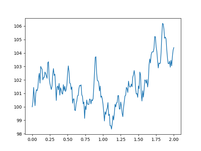
Here we define problem of stock with initial value of 100.0 (say dolars) and
variability of 5% per unit of time (say year) and we simulate it for 2.0
units of time (say years), with default time step of 0.01 (say years).
The SDEProblem constructor takes two callables (functions) as arguments.
First one decribes the drift term, second one describes the noise term. In
python you can define functions either by using def keyword or on-the-fly
using lambda keyword like we did here.
Simulating vector SDEs
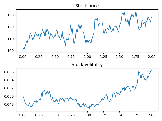
Perhaps you’d want a more complicated model of the market such as GARCH stochastic volitality. In this model stock volitality is described by another stochastic differential equation:
where \(\theta\) controls volitatility mean reverting timescale, \(\omega\) controls typical value of volitaility, \(\xi\) controls variability of the volitaility and \(dW'\) is another source of randomness.
Within this model we have to interconected random processes so we need a vector valued integrator to integrate them simultaneously.
We need to solve the following system of SDEs:
We’ll put stock price in first component of our solution vector x[0] and
volitaility value in the second component of our solution vector x[1].
import pychastic
import jax.numpy as jnp
theta = 0.1; omega = 0.05; xi = 0.1; mu = 0.01
problem = pychastic.sde_problem.SDEProblem(
      lambda x: jnp.array([mu, theta*(omega - x[1])]),
      lambda x: jnp.array([[jnp.sqrt(x[1])*x[0],0],[0,xi * x[1]]]),
      x0 = jnp.array([100.0,0.05]),
      tmax = 2.0
      )
solver = pychastic.sde_solver.SDESolver()
trajectory = solver.solve(problem)
import matplotlib.pyplot as plt
fig, axs = plt.subplots(2)
axs[0].plot(trajectory['time_values'],trajectory['solution_values'][:,0])
axs[1].plot(trajectory['time_values'],trajectory['solution_values'][:,1])
axs[0].set_title('Stock price')
axs[1].set_title('Stock volitality')
plt.tight_layout()
plt.show()
Note that VectorSDEProblem supports driving two equations with the same
noise because of that we needed to pass a diagonal matrix as noise term
description: each noise source is driving the respective equation.
Now suppose we want to price european call option with such model of the market. We can simply simulate lots of trajectories and take expected payout at expiration time.
Because of jit magic it’s much faster to generate all trajectories at once
rather than one at a time. Method solve_many is just what we need here.
import pychastic
import jax.numpy as jnp
theta = 0.1; omega = 0.05; xi = 0.1; mu = 0.01
problem = pychastic.sde_problem.SDEProblem(
      lambda x: jnp.array([mu, theta*(omega - x[1])]),
      lambda x: jnp.array([[jnp.sqrt(x[1])*x[0],0],[0,xi * x[1]]]),
      x0 = [100.0,0.05],
      tmax = 2.0
      )
solver = pychastic.sde_solver.SDESolver()
n_traj = 100 # number of monte-carlo runs
trajectory = solver.solve_many(problem,n_traj)
final_values = trajectory['solution_values'][:,-1]
strike = 120.0
call_payouts = jnp.maximum(final_values - strike,jnp.zeros_like(final_values)) # max(S-K,0)
call_pricing = jnp.mean(call_payouts)
call_pricing
3.76
If you change n_traj from 100 to 1000 you’ll notice that computation
time increased only a litle bit, not 10 fold. This is because of jit
compilation taking some time but happening only once at the beginning.
You’re good to go! There are many options that control the integration precision and speed. You can choose different algorithms for integration as well.
For comprehensive (600 page long) book on the topic try Numerical Solution of Stochastic Differential Equations P. Kloden & E. Platen; Springer (1992)